One question that has been raised in the Interpine team in our LiDAR analysis work is;
“Just how important is the co-location of the LiDAR and ground survey plots ?”
“and hence how much do we have to spend on a GNSS/GPS receivers for fixing LiDAR ground control plots”
Prior to deployment of our upgraded GNSS units in April 2012, in our Interpine LiDAR related ground plots work we have been using the Trimble ProXT GPS receivers. Using these units in dense canopy forest environments, and post processing data collected, provides us with results from 0.7 to 2.5m precision (Confidence Level of 68%). To achieve these levels the field crews must raise the receiver to 5 metres above the ground as well as collecting a minimum of 500 points. It takes between 20 minutes and 4 hours to collect that many points in the NZ Plantation Forest Environment (although this has significantly improved with the upgraded GNSS hardware).
To seek the answer to the above question and understand the hardware requirements to provide productive fixing of plot locations, Interpine carried out a small study to looking at how the strength of the relationship between different LiDAR metrics and total tree volumes changes as the potential error in the co-location increases. The data for the study was selected from a total 124 plots established throughout New Zealand. For every plot, the LiDAR elevation metrics; 30th and 95 height percentile from LiDAR data were calculated. The total tree volume was calculated from the tree level data collected from a field ground survey of these plots.
To understand what affect the accuracy of center plot location has on the relationship between these LiDAR metrics, new plots were created around of the original one. The original plot center was moved randomly with different errors ranging between 0.5m to 25m in the x and y directions with intervals of half meter, furthermore every error was simulated 30 times. For all the simulated plots the same metrics from LiDAR data were computed and the relationship was made with the original volume to see how the displacement of the center plot affected the volume relationship. The following graphs (Figure 1) show an example of the different relationships between original plot data (Graph A) and the new plot data with an error at the extreme end of 25m (Graph B).


Figure 1: Example of a single simulation result with Graph A = high grade fix (no/or little assumed error), Graph B = outer limit of study position simulated error of 25m
The R squared was computed for each error level and for every simulation. The comparison graphical comparison of the R squared values is given in Figure 2.
Figure 2: R-squared variations through simulation of geo-location error of LiDAR vs ground plots (example of P30 LiDAR metric).
The previous figure shows for each 0.5m increment of geo-location error (from 0.5-25m) across 30 simulations there were plots that always had the same or similar R squared, irrespective of plot centre location, most probably where forest characteristics were homogenous. Of particular concern was the somewhat wider random spread of effect when the accuracy was >5m, in other words it was not a continuum of increasing effect from 0.5 to 25m, but more of step variation when geo-location error moved above 5m.
A clear example is showed in Figure 3 where the center plot error in top photo was not so important for the study of the volume in this plot because it was in a homogenous forest, by contrast, for example in the bottom photo the geo-location error can significantly change the result in the inventory process and resulting relationships of LiDAR metrics to ground measurements.
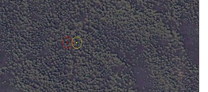
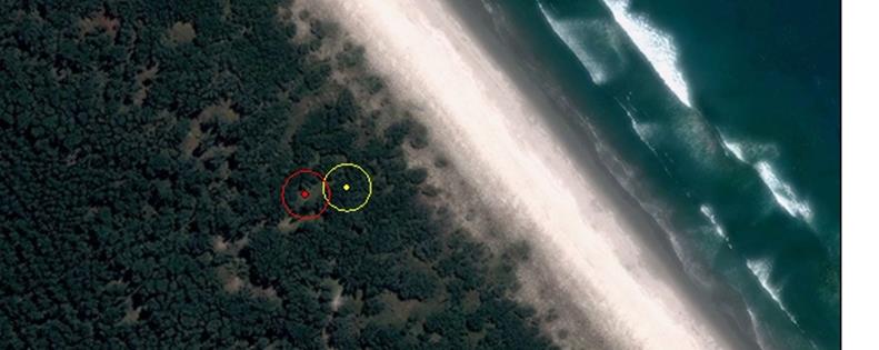 Figure 3: Top shows a homogenous forest with a 25m error, vs the bottom photo showing a heterogeneous forest with a 25m.
In conclusion, locating the correct plot center in the correct position with a GNSS/GPS device has more effect on the study results in the heterogeneous forests environment. Also it was observed that the plots which fell as outliers far away on the trend line were located in heterogeneous areas or even partially on the forest boundary. A pronounced change was shown for all forest types when accuracy was >5m. It is hard to estimate the level of homogenous forest type you will have prior to a survey even in plantations forests.
The advice is to expend the necessary time/resources to locate accurately the center plot with a precision of <2.5m (confidence level of 68%) for all forest types with survey grade GPS units. This should ensure you receive an accurate geo-location within 5m. To do this under a forest canopy you will require a survey grade GPS rated for open environment post-processed precision of submeter.
We welcome input on this project if you are interested in contributing to this work.