Woodlot valuation are traditionally based on averages which tend to ignore the effects of variability or risk. Sources or variability in woodlot valuations typically included the following:
- Log price changes
- JAS conversions factors
- m3 / tonne conversion factors
- Yield analysis – Total Recoverable Volume together with its PLE
- Yield analysis – Log grade mix and their PLE
A method for accounting for this risk is to make use of Monte Carlo simulation technique. The Monte Carlo simulation is especially helpful when there are several different sources of uncertainty that interact to produce an outcome.
Monte Carlo simulation performs risk analysis by building models of possible results by substituting a range of values (probability distribution) for any factor that has inherent uncertainty. It then calculates the results over and over, each time using a different set of random values from the probability functions. Monte Carlo simulations sample probability distribution for each variable to produce thousands of possible outcomes. Rare samples are selected from very low probability regions whereas most likely samples are selected from high probability regions. The results are analysed to get a probability distribution of possible outcomes.
Various packages are available as Excel add on which efficiently handle Monte Carlo simulations. These include Oracles “CRYSTAL BALL” and Frontline Systems Inc “RISK SOLVER PRO”. This example is done using Risk Solver Pro. The example shown below is just a simplified valuation just to add context and some element of reality. All numbers adjusted from reality and should not be used for any other purposes except this demonstration of concept.
Simple Woodlot Valuation Example
A 20 year old 22.2ha P.radiata woodlot in had a 2.5% PHI inventory carried out. A typical valuation is typically conducted using averages. An example valuation is shown in the spreadsheet in figure 1 below. This woodlot valuation example inventory yield analysis calculated a total recoverable volume (TRV) of 554.6m3/ha with an associated log grade mix. Log prices MPI 12Q rolling average. These prices are provided in JAS m3 F.O.B. Typical JAS conversion factors and wharf fees are applied to get a standard m3 A.W.G. price. Variable harvesting, transport, and management fees are converted using a typical m3/tonne conversion factor. In this case for a 0.98m3/tonne conversion was applied. A fixed road access and landing construction fee was applied.
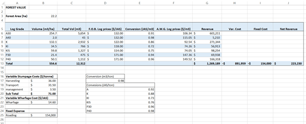
Figure 1: Simplified spreadsheet woodlot valuation calculation.
In this case study the woodlot has a value of $223,230.
Log price Variability
Export log prices are subject to monthly changes driven largely by port inventories and demand. For this example we will just focus on export market. Log price variability is shown in the graph below. Figure 2 below provides a look at the historic log price movements.
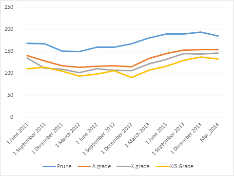
Figure 2 – MPI Quarterly Log price Survey
Using this price variability a probability curve for each log grade can be developed
| Log grade | MEAN | STD DEV |
| Pruned | 171.29 | 15.65 |
| A Grade | 131.88 | 16.40 |
| K Grade | 121.96 | 16.87 |
| KIS | 111.46 | 15.08 |
Table 1 – Log price statistics.
Based on the log price change a price probability curve can be generated for each log grade based on the mean price and standard deviation. Figure 3 below provides a price probability curve for A grade logs.
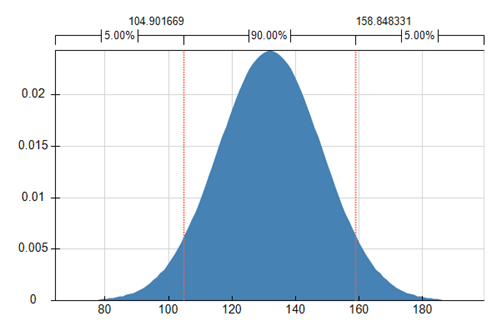
Figure 3 – A log grade price probability curve based on a Normal Distribution.
Similar probability distributions can be developed for each log grade price. In addition JAS m3 per tonne conversion factors can also modelled into probability distributions as shown table 2.
Table 2 – JAS m3/ tonne conversion rates for a 20yr old stand delivered to Marsden point.
|
Row Labels |
Average of Conversion | StdDev of Conversion | Max of Conversion |
Min of Conversion |
| A | 0.92 | 0.05 | 1.00 | 0.81 |
| K | 0.88 | 0.05 | 0.99 | 0.77 |
| KI | 0.73 | 0.08 | 0.84 | 0.64 |
| KIS | 0.76 | 0.05 | 0.85 | 0.68 |
| P30 | 0.96 | 0.05 | 1.03 | 0.88 |
| P40 | 0.98 | 0.03 | 1.03 | 0.92 |
| Grand Total | 0.88 | 0.09 | 1.03 |
0.64 |
Based on these figures a normal probability distribution is fitted to each log grade JAS m3/tonne conversion factor. A m3/tonne conversion factor is also applied.
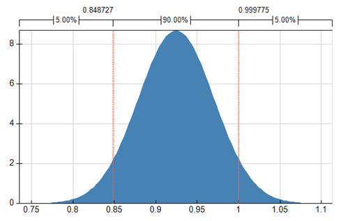
Figure 4 – A grade JAS m3/tonne Conversions.
Similar probability distributions are fitted for each grade conversion.
Volume and Grade Mix Variability
YTGen yield analysis reports provide a TRV by log grade for inventory data. Table 2 below provides the YTGen yield analysis summary report for the woodlot case study.
Table 3 – YTGen yield analysis summary report.
| Age | GradeName | TRV | VolumeStdError | PLE |
| 20.57949 | A30 | 254.7 | 31.11442 | 28.9% |
| 20.57949 | A40 | 2.0 | 2.039839 | 236% |
| 20.57949 | K | 132.1 | 13.77265 | 24.7% |
| 20.57949 | KI | 34.5 | 5.232425 | 35.8% |
| 20.57949 | KIS | 59.8 | 6.027756 | 23.85 |
| 20.57949 | P30 | 21.4 | 5.897073 | 65.2% |
| 20.57949 | P40 | 50.1 | 11.82521 | 55.8% |
| 554.6 | 42.75081 | 18.2% |
Based on this information a probability distribution for each log grade recoverable volume can be generated. Volume standard error is converted to Standard deviation and a normal distribution fitted. Figure 4 below provides an example of A_30 grade volume probability distribution curve.
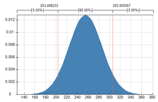
Figure 4 – Volume per ha of A_30 grade (Normal Distribution).
Grade mixes are used to determine the weighted average log price (grade mix). Total Recoverable Volume probability curves are used for used in calculating the stumpage per ha. See figure 5.
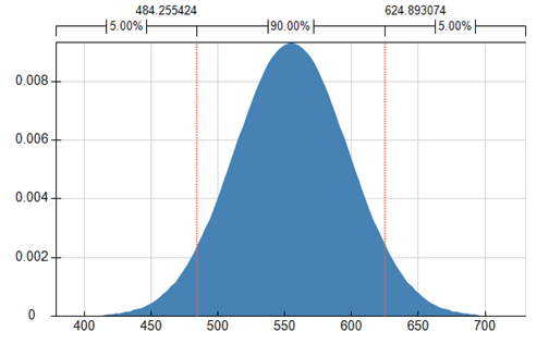
Figure 5 – Total Recoverable Volume per ha (Normal Distribution)
Costs
Roading access costs are considered fixed based on an engineering quote provided for the woodlot. In this case study a total engineering cost of $154,000 was applied to the valuation.
The following variable cost are applied to the woodlot valuation.
| Variable Stumpage Costs ($/tonne) | |
| Harvesting | $ 36.00 |
| Transport | $ 31.50 |
| management | $ 3.50 |
| Sub Total | $ 71.00 |
| Variable Wharfage Cost ($/JAS) | |
| Wharfage | $ 14.60 |
Volume weight conversion factor
Variable stumpage costs are based on tonne basis and are charged out over weigh bridge figures. These costs need to be converted to volume base for valuation purposes. Conversion rates for m3/tonne vary throughout the year. Figure 6 below show the season change in conversion rates.
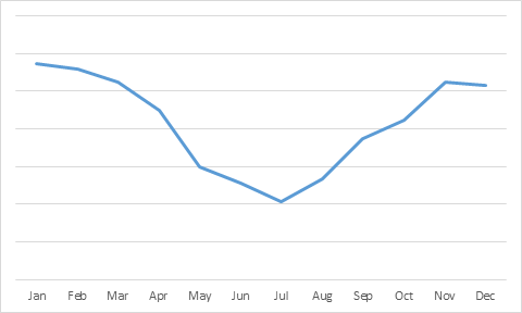
Figure 6 – Seasonal m3/tonne Conversions
A normal distribution for this conversion factor is not the best fit and a straight line even probability distribution is fitted to this conversion factor.
Results
Risk Solver Pro was used as a Monte Carlo simulation software package.
10,000 valuation simulations were run selecting random points along each variable probability curve. The results of the 10,000 simulations are provided in Figure 8 below.
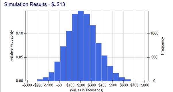
Figure 8 – Results of 10,000 woodlot valuation simulations. Summary statistic for the simulations are shown below:
| Statistics | |
| mean | 218,305 |
| Standard Deviation | 147,281 |
| Mode | 206,999 |
| Min | -319,398 |
| Max | 833,926 |
| Range | 1,153,324 |
Although the mean of the simulation ($218,305) is close to the standard averaging method of valuation calculation ($223,230), the likely hood that the woodlot value could be significantly different is large. We could say we are 90% confident the woodlot value is likely to fall between $0 and $450,000.
Huh what did you say ! ok this is an extreme example, but we just wanted to show you how important it is to consider risk in a woodlot valuation. Don’t just expect one number to be the correct one !
Sensitivity Analysis
A sensitivity analysis is carried out to determine which variable has the greatest impact on the value of the woodlot. Figure 9 below shows that the greatest impact on this woodlot case study value is attributable to the m3/tonne conversion ration followed by the log prices, hence the actual timing and length of time the harvest spans contributes in this case to the greatest risk.
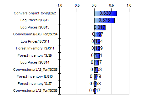
Figure 9 – Woodlot valuation Sensitivity Analysis
So need to consider risk in your woodlot valuation, talk to our consulting team.