David Herries recently presented at ForestTech 2014 an overview of Plot Imputation as a method for development of forest yields using YTGEN. The presentation was designed to introduce and simplify the concepts of k-nearest neighbour and plot imputation while outlining LiDAR’s role in providing descriptive cloud metrics. The following yield calculation pathway was introduced as outlined in Figure 1;
Figure 1: yield calculation pathway for plot imputation.
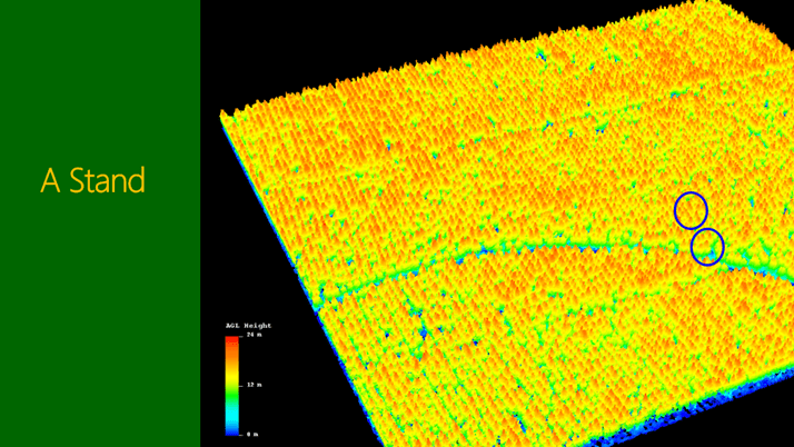
To help understand point clouds and their link to and use in forest product yield tables we need to be confident the first unit of measurement: a tree. In Figure 1, 2 and 3 show where two trees are extracted from a stand and used to explain the point cloud and the metrics derived from them. The two trees, both from the same stand, 50m from each other. The first is close to the road, therefore an edge tree, unpruned and clearly a heavy branching habit. The second being within the stand and pruned. So what is the point cloud telling us and how do we assess it. A couple examples of metrics is shown, being bincentiles or height bins as a % of total height, and percentiles (heights of a % of points).
Figure 1, 2 and 3 A look at two different tree forms and a couple of methods used to quantify the LiDAR discrete return descriptive metrics.
These metrics can then be done across a reference plot as shown in Figure 4. This introduced to the attendees the concept of “Reference Plots”. These being a ground measured plot where known assessments of volume and grade mix have been conducted, and a yield table is developed in software such as YTGEN.
Then it is important to understand that these same metrics can be calculated across the entire stand or forest in a grid of cells say 25m in size. This is then referred to as the “Target Imputation Grid”. The grid cells will often match a similar area to the reference plot size, albeit square instead of circle in this particular example. This same grid also ends up being a “GIS raster” across the forest area.
Figure 4 and 5 shown the same metrics being calculated for a square grid cell.
Using the forest yield reference plots and their respective metrics, selection of the LiDAR metrics which have the largest impact on the yield estimates is done. It is important to note that at this stage we often introduce “non LiDAR metrics” such as stand age or anything else we might know about both the reference plots and the target imputation grid forest attributes.
Figure 6 modelling is used to select an optimal set of predicator variables.
Once the predictor metric relationships are established the reference plots are related (imputed) to represent a grid cell across the Target Imputation Grid (Figure 7). This introducing the concept of nearest neighbours (kNN). In the simplest sense this could be thought of as 1 plot is used to represent each grid cell in the network, that being often referred to k=1 in the terminology of kNN. However we can use more than 1 plot to represent a grid cell (k=2,3,4 etc.) as a simple average or provide a respective weighting of each of these plots for each grid cell when k>1.
Figure 7 allocating the nearest neighbours
Then it’s just maths to simple select any “Area of interest” (typically a stand, harvest area or might be an entire forest!) and the respective target imputation grid cells that fall in the area, to get a final yield table (Figure 8). And of course the core difference in “Plot Imputation” is the fact that for any area of interest it might be that not a single reference plot needs to fall into that area.
Figure 8 Calculating yield from any Area of Interest (AOI).
The Interpine team, having been working with Plot Imputation for prediction of Forest Yield for several years now, felt there was not enough transparency about this pathway, and people commonly ask and are confused about yield raster’s and LiDAR metrics, kNN, areas of interest, the importance of reference plots and imputation. This presentation was focused on re-igniting interest in LiDAR within the resource forester community within NZ and Australia, and hopefully inspire some further adoption of LiDAR for resource inventory.
If you would like a copy of the full presentation you can download it here:


